Microsoft Excel XP package
Microsoft Excel XP application is designed to perform tabular calculations in solving a wide range of economic, statistical, scientific, scientific-technical and many other tasks. It is often the fastest and most acceptable way to automate both tabular and conventional calculations that accompany the fulfillment of relevant sections of academic works. 
The application is integrated into the general Microsoft Office XP package, which includes several functionally different applications (Microsoft Word XP text editor, Paintbrush graphic editor, Power Point XP presentation editor, etc.), but with a similar interface. Work in all Microsoft Office XP applications is unified.
Spreadsheet Elements
When Microsoft Excel XP application is launched for execution, a new application document is created in the form of a spreadsheet (Fig.1). The spreadsheet is organized into elements called table cells. A cell is identified by the row and column at the intersection of which it is located. Columns are named with single letters of the Latin alphabet or their combination (A, C, AA, ABC, etc.), rows are numbered.
Therefore, to uniquely determine the address (location) of a cell in the table, it is enough to specify the name of the column and the number of the row at the intersection of which it is located. For example, A6, K12, A2, B12, etc. The number of cells (rows and columns) in the table is limited only by the computer memory. 
Sometimes it is necessary to set an absolute (unchangeable) cell address. For this purpose, the monetary unit sign $ is used. If it is written before the column name, row number, or both, the corresponding elements of the cell address will not change when copying. Such an entry can be $O12, O$12 or $O$12.
The table cell where the cursor is located is called the active cell. It is the only cell where you can create or edit something. To make it easier to orient where the cursor is located, the active cell is highlighted with a thickened frame.
The rectangular area of active cells is called a block. To create a block, press the left mouse button and move the cursor over the table cells. Another variant of block selection: press the "Shift" key and move the cursor with the mouse or with the cursor keys.
The block is highlighted in black color (all cells are darkened except the one from which the block creation was started). A block is de-selected by moving the cursor to another place in the table or by creating a new block. As long as the block is selected, it can be operated as a single object.
Entering information in Excel
To enter information into any cell of the table, make it active (move the cursor to it with the mouse or keyboard keys), type a string of characters (numbers, letters, special characters) and press Enter or the cursor key.
If it is necessary for the string of input characters to be perceived as a number, it must not contain any characters other than digits, the "+" or "-" sign and separators: a) comma separating the integer part of the number from the fractional part; b) Latin letter E separating the exponent of the degree from the base in the exponential form of number recording.
To enter a formula, type the "=" sign followed by the formula itself without a space, taking into account the conventions for writing it. Whenever a character string cannot be identified as a number or formula, it is treated as text.
Excel Cell Format
To present the information contained in a cell in the desired form give the "Format Cells" command - press the right mouse button and select this command from the context menu that appears.
Another option - use the sequence of commands "Format" "Cells" from the text menu (Fig. 2). In addition, many actions specified from the submenu of the "Format Cells" command can be performed using the corresponding toolbar buttons. 
The dialog box of the "Format Cells" command (Fig. 3) has six tabs, in each of which parameters are grouped to set the way of interpreting the information and colorful design.
For example, if a cell contains a set of digits that make up a number, then in the "Number" tab you can define the way of perceiving this number - as a number written in decimal or exponential form, date, time, text, etc. In the other tabs you can specify the way of aligning data within one or a group of cells, select a font for writing characters, define the shape of cell borders, etc. 
You can set format parameters not only for one active cell, but also for several cells at once. To do this, first select the desired group of cells as a block and give the "Format Cells" command.
For more information, see the Microsoft Excel 2003 Help.


